<< Part II | This is Part III of a multi-part series on Bitcoin block propagation with IBLT. | Part IV >>

I want to get idea on how failure probability, the probaility that decoding of the IBLT fails, depends on cellCount. So the question is

How fast does failure probability drop when the IBLT size increase?

To answer this, I encoded a certain amount of differences (equal amount of absent and extra transactions), where the transactions were selected randomly from a 1000 block span on the blockchain. The IBLT is then decoded to see if it succeeds or fails. The process is repeated 10000-100000 times with new random transactions in each sample. I did the same test for seven different diff cell Counts for 6 different (32-1024) diff counts.

for i = 0..5 // For each diff count
    diffCount = 32 \* 2^i
    cellCount = findGoodStartValue()
    for j=0..6 // For each cell count
        cellCount = calculateStep() // Some arbitrary step
        samples = j > 3 ? 100000 : 10000
        for k=1..samples // For each sample
            extra = select diffCount/2 random transaction
            absent = select diffCount/2 random transactions not in extra
            runSample(cellCount, extra, absent)

Enough said, here are the graphs:

We note here that the more differences we have, the more linear the graph. At least for the interesting span between failure probability 0.1 and 0.001. If we plot this data as failure probability vs cost in bytes per diff, I call it "diff cost", we can see an interesting pattern:

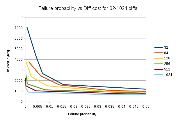
The first observation is that the diff cost decreases as the number of diffs increases. For example, at failure probability 0.02 the diff cost is roughly 1500 bytes if we have 32 diffs, but if we have 1024 diffs, the diff cost is around 700 bytes.

The other thing we notice is that as failure probability approaches 0, the diff costs gets more spread out. At failure probability 0.005, the 32 diffs diff cost is on the order of 4000 bytes, while the diff cost for 1024 diffs is roughly 900 bytes.

Given this, it looks like we shouldn't aim for a certain failure probability at all times, but rather select a failure probability that is suitable for the estimated amount of diffs we have. For 32 diffs, the sweet spot seems to be around 0.015, for 128 diffs it seems to be around 0.01 and for 1024 diffs its about 0.001.

That's it for this time. In Part IV we will indulge in diffCount VS failureProbability. What happens when you have a fixed IBLT size and increase the number of differences.